Snowflake Scalability & Performance Mastery

---

Mastering Multi-Cluster, Scalability, Warehouse Size & Objects in Snowflake

In the Snowflake ecosystem, true architectural maturity goes beyond knowing how to run queries — it’s about understanding how Snowflake scales, how to size warehouses efficiently, and how multi-cluster compute and objects come together to deliver predictable performance at any scale.

If you’re preparing for the SnowPro Core certification or designing enterprise data solutions, this tutorial will help you build a strong foundation across four critical Snowflake domains:

1. Multi-Cluster Warehouses
2. Scalability in Snowflake
3. Warehouse Size — Configuration & Performance Nuances
4. Snowflake Objects (tables, micro-partitions, stages, file formats, streams, tasks, and views)

Let’s explore each one in detail — with practical examples, pro tips, and common pitfalls to avoid.

---

Section 1 — Multi-Cluster Warehouses

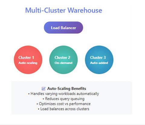
What Are Multi-Cluster Warehouses?

A Multi-Cluster Warehouse (MCW) in Snowflake enables horizontal scaling — adding more clusters in parallel to handle concurrent workloads. In contrast, vertical scaling increases the size of a single warehouse (e.g., Small → Medium → Large).

MCWs are essential when your workload experiences sudden query spikes or supports high-concurrency business intelligence (BI) users. They ensure that user queries are distributed evenly across clusters, reducing queue time and maintaining consistent performance.

Typical use cases:

• High-concurrency dashboards (e.g., hundreds of Tableau or Power BI users)
• Multi-tenant SaaS analytics platforms
• End-of-month reporting or marketing campaign spikes

Configuring a Multi-Cluster Warehouse

You control an MCW with two parameters:

• MIN_CLUSTER_COUNT — minimum number of clusters that remain active
• MAX_CLUSTER_COUNT — maximum clusters that can spin up automatically

You can also set the scaling policy to AUTO (scale up/down dynamically) or ECONOMY (scale down faster when load drops).

ALTER WAREHOUSE BI_WH 
  SET MIN_CLUSTER_COUNT = 1, 
      MAX_CLUSTER_COUNT = 3, 
      SCALING_POLICY = AUTO;

Cost vs Performance Example:
Suppose your Large warehouse consumes ~8 credits/hour. Setting MAX_CLUSTER_COUNT = 3 allows Snowflake to scale up to 3 clusters (≈ 24 credits/hour at peak). This flexibility eliminates query queuing during high-load periods, then scales back to one cluster when demand drops — optimizing cost per throughput.

Pro Tip:

Monitor concurrency and auto-scaling history in the WAREHOUSE_HISTORY view. Start with MIN=1, MAX=2, and gradually tune up as usage patterns become clear.

Common Mistake:

Setting MAX_CLUSTER_COUNT too high without monitoring workload — this can trigger unexpected cost surges if spikes are frequent or sustained.

---

Section 2 — Scalability in Snowflake

Vertical vs Horizontal Scaling

Snowflake achieves elasticity by separating compute, storage, and cloud services:

• Vertical scaling — increase warehouse size to allocate more CPU, memory, and I/O to a single cluster.
• Horizontal scaling — increase the number of clusters (MCW) to process concurrent workloads in parallel.

Because compute and storage are independent, you can scale up or out on demand — without impacting stored data or system metadata.

Key Scalability Patterns

1. Workload Isolation:
Run ETL, BI, and ad-hoc analytics in separate warehouses to avoid contention.

2. Resource Monitors:
Create monitors to track credit usage and automatically suspend warehouses that exceed limits.

3. Auto-Suspend / Auto-Resume:
Suspend inactive warehouses after 5–10 minutes to minimize idle cost; resume instantly when queries arrive.

Decision Framework

Symptom	Recommended Action
Queries slow with few users	Scale Up (increase warehouse size)
Queries queue under heavy concurrency	Scale Out (enable Multi-Cluster)
Queries slow despite scaling	Optimize SQL / Data Layout

Real-World Scenario

A retail organization runs nightly ETL (00:00–03:00) and experiences heavy BI traffic between 08:00–11:00.

Strategy:

• ETL → Dedicated Medium warehouse.
• BI → Large Multi-Cluster (MIN = 1, MAX = 3).
• After 11:00 AM, all warehouses auto-suspend.

This architecture handles concurrency efficiently without waste.

Scalability Checklist

• Use workload-specific warehouses.
• Combine auto-suspend/resume with resource monitors.
• Monitor query history for queuing trends.
• Regularly review credit consumption by warehouse.

Pro Tip:

Elasticity is Snowflake’s superpower — but discipline around sizing and suspension policies is what makes it affordable.

Common Mistake:

Using a single oversized warehouse for all workloads; it simplifies admin but destroys cost efficiency and predictability.

---

Section 3 — Warehouse Size : Configuration & Performance Nuances

Understanding Warehouse T-Shirt Sizes

Each size doubles compute resources from the previous one. Approximate relative capacities are consistent across cloud regions, but actual credit rates vary by edition and region.

Size	Relative Compute	Typical Use Case
X-Small	1×	Development, small ad-hoc
Small	2×	Light ETL, testing
Medium	4×	Standard ETL, moderate analytics
Large	8×	High-concurrency dashboards
X-Large	16×	Enterprise BI workloads
4X–6X Large	64–128×	Heavy aggregation / ML pipelines

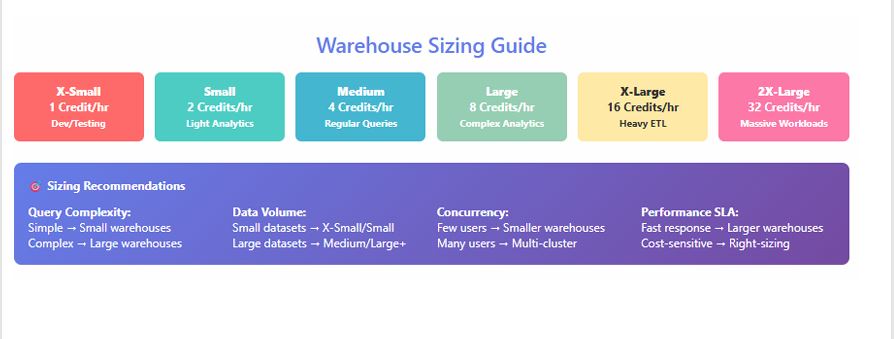
What “Doubling Capacity” Means

Moving from Medium → Large roughly doubles CPU cores and I/O throughput. Query runtime may drop 40–70 %, but credit consumption per hour doubles — so optimization is key.

Credit Usage Patterns

Warehouses consume credits per second of active compute, with a minimum 60 seconds per start. Auto-suspend after 5 minutes inactivity is often ideal for shared BI warehouses.

Micro-Benchmarking Approach

1. Choose representative queries.
2. Execute on Medium, record average runtime and credits.
3. Repeat on Large and 2X-Large; compute % improvement vs credit delta.
4. Identify diminishing returns: if doubling size yields < 15 % gain, keep smaller size.

Performance Optimization Checklist

• Review QUERY_HISTORY for queuing and execution patterns.
• Enable auto-suspend/resume per warehouse.
• Use result caching for repetitive queries.
• Partition workloads logically — don’t mix ETL with BI.

Pro Tip:

Start small, measure, scale gradually. Real optimization is about observability, not assumptions.

Common Mistake:

Over-provisioning “just in case.” It doubles spend with marginal benefit; use data-driven benchmarks instead.

---

Section 4 — Snowflake Objects

Snowflake’s logical and physical objects form the foundation of your data ecosystem. Understanding how each works — and interacts with storage and compute — is essential for tuning performance and minimizing cost.

Databases & Schemas

Logical containers for grouping related data objects.

CREATE DATABASE SALES_DB;
CREATE SCHEMA SALES_DB.RAW;

When to Use: Organize data by domain or environment (e.g., RAW, STAGE, PROD).

---

Tables (Permanent, Transient, Temporary)

• Permanent: Long-term, protected by Time Travel and Fail-Safe.
• Transient: Lower cost, no Fail-Safe; good for staging.
• Temporary: Session-scoped, auto-drops at session end.

CREATE TRANSIENT TABLE STG_ORDERS AS SELECT * FROM RAW.ORDERS;

When to Use: Transient for ETL intermediates; Temporary for scratch computations.

---

Micro-Partitions & Clustering Keys

Snowflake stores data in 16 MB micro-partitions. Efficient clustering ensures query pruning and faster scans.

ALTER TABLE SALES ADD CLUSTER BY (REGION_ID);

When to Use: Add clustering only for large tables (> 100 GB) frequently filtered by specific columns.

---

Stages (Internal & External)

Define file storage locations for loading/unloading data.

CREATE STAGE mystage URL='s3://mybucket/data/';

When to Use:

• Internal for small/local loads.
• External for enterprise data lakes (S3, Azure Blob, GCS).

---

File Formats

Reusable objects defining structure of staged files.

CREATE FILE FORMAT mycsv TYPE = 'CSV' FIELD_DELIMITER = ',' SKIP_HEADER = 1;

When to Use: Standardize ingestion definitions across pipelines.

---

Streams (Change Data Capture)

Tracks inserts, updates, and deletes on tables.

CREATE STREAM STRM_ORDERS ON TABLE RAW.ORDERS;

When to Use: Real-time incremental processing and replication.

---

Tasks (Scheduled Automation)

Runs SQL statements or pipelines on schedule.

CREATE TASK TASK_ETL
  WAREHOUSE = ETL_WH
  SCHEDULE = 'USING CRON 0 * * * * UTC'
AS
  CALL LOAD_ORDERS();

When to Use: Automate recurring transformations and CDC merges.

---

Views & Materialized Views

• Views: Virtual; recomputed each query.
• Materialized Views: Physically stored, auto-refreshed for faster reads.

CREATE MATERIALIZED VIEW MV_SALES AS 
SELECT REGION, SUM(AMOUNT) FROM SALES GROUP BY REGION;

When to Use: Materialized Views for heavy aggregation tables accessed frequently.

---

Pro Tip:

Maintain consistent naming (DB.SCHEMA.OBJECT), cluster only when necessary, and manage small files via staging merges.

Common Mistake:

Over-clustering or leaving tiny staged files uncombined — both degrade load performance and inflate cost.

---

Summary & Key Takeaways

• Multi-Cluster Warehouses enable concurrency without queuing by scaling horizontally.
• Scalability in Snowflake combines compute elasticity and workload isolation for predictable performance.
• Warehouse Sizing determines cost efficiency; benchmark and right-size using data, not guesswork.
• Snowflake Objects (tables, stages, streams, tasks, views) are the building blocks — design them intentionally for speed and maintainability.

Together, these four areas form the operational backbone of every performant Snowflake deployment.

---

Next Steps / Resources

• Read official documentation on Multi-Cluster Warehouses, Performance & Scaling, and Working with Objects.
• Hands-on lab ideas:
  • Create a multi-cluster warehouse and simulate concurrent queries.
  • Benchmark Medium vs Large warehouses for the same workload.
  • Explore micro-partition metadata with SYSTEM$CLUSTERING_INFORMATION().
• Continue with SnowPro Core Certification Guide for deeper coverage of performance, scalability, and architecture.

---

This Snowflake Scalability Guide equips you with the conceptual clarity and operational discipline needed to manage cost, concurrency, and compute performance — the exact skills that separate proficient users from Snowflake power architects.